Decision Trees With Gradient Descent

Decision trees are a commonly used machine learning technique. They often are preferred to neural networks or more complex models for small problems that wouldn’t need deep learning; libraries implementing decision tree “forests” trained via gradient boosting like XGBoost and CatBoost are some of the most popular ML frameworks out there.

A decision tree generally works as follows: given your input feature vector $\v{x}$, each binary node $i$ computes a linear function $\v{v}_i\cdot\v{x}+b_i$. If this comes out > 0, go one side, otherwise go the other. Once you’re at a leaf, you can read out its related outcome, and that’s your answer. There are variations; forests for example aggregate multiple trees to obtain a more robust judgement. But the core principle stays the same.

The main difficulty with building a decision tree is in the training process. The nature of the tree is discontinuous, as you need to keep appending nodes progressively as you build the tree in depth. This isn’t a process you can differentiate, and appropriately, trees aren’t trained via gradient descent, and instead are built with other methods, such as greedy recursive binary splitting (as in the CART algorithm).

But what if… you could actually do it?

(Note: the following work is based on an idea I originally had by myself, then found out it overlapped significantly with Frosst & Hinton’s Distilling a Neural Network Into a Soft Decision Tree. I haven’t re-read that paper in a while now and rebuilt the model still mostly from my own intuitions so it’s probably not 1:1 identical, but it’s been influenced by that work)

Trees are logistic regression?#

Consider a simple binary tree with depth 2: one node $O_0$, bifurcating to two more nodes $O_1$ and $O_2$, and then four leaves $L_0$ to $L_3$. Let’s now treat this as a soft tree, meaning, a tree in which each passing sample merely has a probability of going to the left or right. By convention, at node $O_i$, we make the logit of the probability of going left $0$, and the logit of the probability of going right $r_i = \v{v}_i\cdot\v{x}+b_i$. Therefore the actual probabilities are:

$$ P_i(\mathrm{left}) = \frac{1}{1+e^{r_i}} $$

$$ P_i(\mathrm{right}) = \frac{e^{r_i}}{1+e^{r_i}} $$

What paths can a sample take? There are four possible:

• $O_0$ -> left -> $O_1$ -> left -> $L_0$
• $O_0$ -> left -> $O_1$ -> right -> $L_1$
• $O_0$ -> right -> $O_2$ -> left -> $L_2$
• $O_0$ -> right -> $O_2$ -> right -> $L_3$

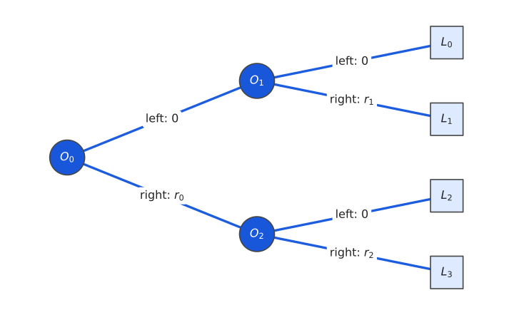
Probabilities multiply, so the unnormalized probabilities of each path will be going like:

• $e^{0}e^{0} = 1$
• $e^{0}e^{r_1} = e^{r_1}$
• $e^{r_0}e^{0} = e^{r_0}$
• $e^{r_0}e^{r_2} = e^{r_0+r_2}$

We can find these with a simple method. Let’s put all the vectors into a weight matrix $V$ and all biases into a vector $\v{b}$. Then:

$$ \v{r} = V\v{x} + \v{b} $$

is the vector of all the right-logits in each node, $\v{r} = (r_0, r_1, r_2)^T$. If we premultiply by a path matrix:

$$ P = \begin{bmatrix} 0 & 0 & 0 \\ 0 & 1 & 0 \\ 1 & 0 & 0 \\ 1 & 0 & 1 \end{bmatrix} $$

we can find an output activation vector $\v{y}$ (component $y_i$ corresponding to leaf $L_i$):

$$ \v{y} = P(V\v{x}+\v{b}) = W\v{x}+\v{q} $$

where we show how this is pretty easily made equivalent to just having a weight matrix $W = PV$ and a new bias vector $\v{q} = P\v{b}$ ¹.

What are the actual probabilities? Well, by the product rule:

$$ P(L_j) = \prod_{i \in \mathrm{path}(j)} \frac{e^{z_i}}{1+e^{r_i}} $$

where $z_i$ will be $0$ or $r_i$ depending on what the path follows. Basically, the argument of the exponential depends on which directions the path actually takes, whereas the denominator merely depends on which nodes it visited.

Built this way, you can have your “soft” tree assigning probabilities to each leaf. You could potentially already use this as a classifier (training on cross-entropy), as long as you’re happy with the constraint that depth $D$ implies exactly $2^D$ classes. In that sense, this is logistic regression albeit with a slightly different activation function ².

However, the constraint is quite restrictive! You can end up forced to build an unbalanced tree if you have a number of classes that aren’t a power of two, and even if they are, that constrains your maximum depth, something that should be more an expression of the complexity of the problem. This is, however, easily fixed by using what Hinton in the paper above calls the “Mixture of Bigots”.

Trees are neural networks?#

The “Mixture of Experts” paradigm has grown quite common in many contemporary large models. It essentially consists of having a block or layer built of many small models (“experts”), as well as one classifier function whose purpose is to mix the outputs of those experts. Essentially, each expert is supposed to learn to solve a certain type of problem, whereas the classifier learns to distinguish between those problems and reroute to the correct expert based on the query. To run with the metaphor, the classifier will put you in contact with a doctor if you ask “what are the symptoms of measles?” and with a lawyer if you ask “how many years does a patent last?”.

What’s the simplest possible “expert” model we can imagine? That would be a constant - something that answers the same thing when called upon no matter what. This is what the Frosst and Hinton paper I cited earlier calls a “bigot”, in reference to how stubbornly unchanging its opinion will be. If we use bigots, the vast majority of the responsibility falls on the classifier, which is essentially forced to pick between a set of predefined answers. We can also see how this generalises our tree structure very well. Suppose we have a classification problem with three classes. Then we couldn’t possibly build a full balanced binary tree with only three leaves. But we could decide an arbitrary depth (for example, $D = 3$, giving us 8 leaves) and then assign to each leaf a “bigot” which is essentially just a vector with three elements (logits or probabilities for the final classes). Given what we’ve said above about logistic regression, you get something like this:

$$ \v{\hat{y}} = B\sigma(W\v{x}+\v{q}) $$

with $B$ being the “bigot” matrix of shape n_classes x n_leaves; $\sigma$ is essentially an activation function, albeit not quite softmax due to the difference in normalization mentioned above. We’ve retrieved what is essentially a regular single hidden layer neural network³! The main difference is that the activation function is unusual and the size of the hidden layer can now have a more well-defined meaning: it’s directly related to the depth of the tree, that is, the number of bigots we’re using. You could for example split a problem into four possible outcomes (tree depth of 2), which would allow some bigots to peak specifically at one class while others identify regions of uncertainty. Increasing the inner size will make the problem more fine grained as we split the space of inputs into more and more domains, each with its own pre-baked answer.

How to grow a real tree#

There remains one thing. If we simply trained this model via cross-entropy loss on a classification problem we would get good results, but most likely, these would leverage significantly some amount of soft mixing between all the leaves of the tree. This is fine if we plan to use this model as is, but given its analogy to a tree, it would be nice if we could use it as a tree, train it with gradient descent but then do inference by going through the nodes along a single greedy path, which would make inference $\mathcal{O}(D)$ instead of $\mathcal{O}(2^D)$. In this mode we would traverse node by node, computing the logit at each node, turning left or right based on whether it’s negative or positive, and repeat until we reach a leaf. For that to be possible, though, we need the tree to be trained not just to give a correct answer, but to do so always by flowing through a specific path.

How to do that? Well, we’ve seen before how to turn the logits for every node into logits for each possible path. We can do that for any subtree, not just the overall tree; let’s call

$$ \v{p}_d = \sigma_d(P_d(V\v{x}+\v{b})) \qquad 0 < d \le D $$

the probability distribution for our path to go through each of the $2^d$ leaves after the first $d$ layers of the tree ⁴. We want this to be as sparse as possible; in a “classic” tree, it will be a vector of zeroes with a single entry set as one. Or in other words, we want it to be a very low entropy distribution. We can then use this as our training loss:

$$ \mathcal{L} = -\sum_i {y_i\log(\hat{y}_i)} -\sum_{d=1}^D \lambda_d \sum_{j=1}^{2^d} p_d^{(j)}\log(p_d^{(j)}) $$

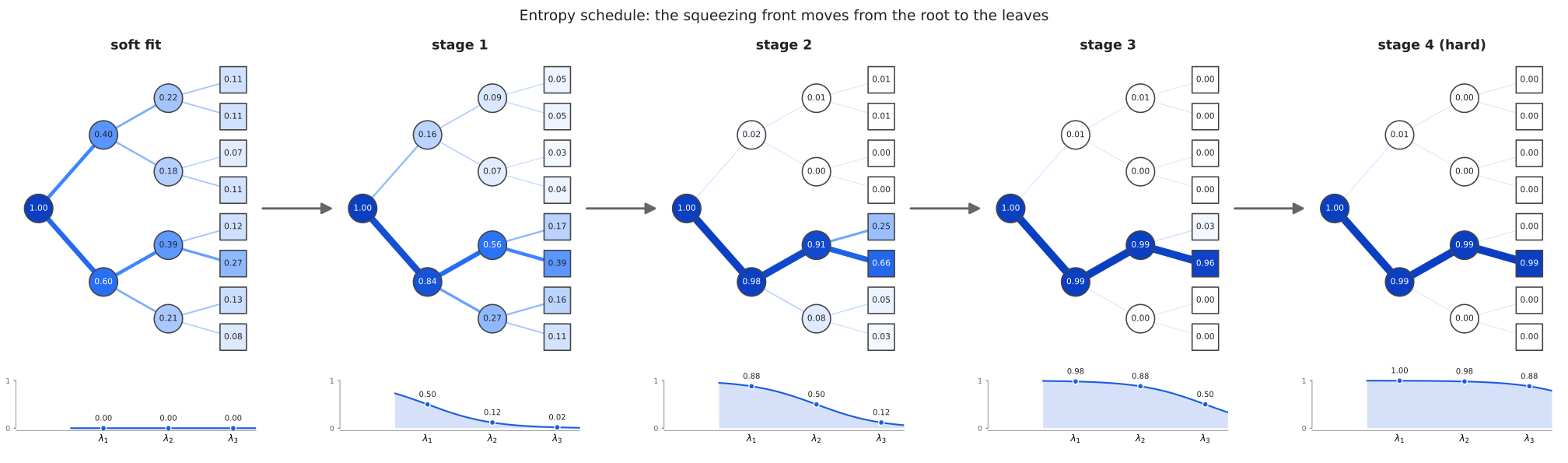
which adds an entropy regularization term for the activations at each layer, with a per-layer regularization strength parameter $\lambda_d$. Since imposing this constraint right away would risk “freezing” the model in an ineffectual shape, we instead “squeeze” the outputs of the tree gradually. We use a schedule that starts with all $\lambda$ being zero, and then begins increasing them from the top down, all the way to the leaves.

Further regularization tricks include applying an L1 regularization to the rows of $V$ (this forces each node to prefer focusing only on a small amount of input features, making them more interpretable) as well applying L2 regularization to $B’$ (the actual unconstrained weights underlying $B$, as discussed in ³).

Try it yourself#

A live example using the classic Iris Dataset can be found here, as a marimo notebook; you can also view it in your browser. To run it yourself, you need uv:

git clone https://github.com/stur86/miniml-examples.git
cd miniml-examples
uv sync
uv run marimo edit examples/mob_tree/mob_tree.py